Stellamorph
Exploring Stellarator Stage I Design with Stochastic Flow Search.
Why Fusion?
Energy is the hidden substrate of modern civilization. Industry, transportation, computation, medicine, and daily life all depend on reliable power. The challenge is therefore not only to produce more electricity, but to produce energy that is clean, safe, affordable, and available when society needs it.
This remains a difficult open problem. Much of today’s useful energy is still tied, directly or indirectly, to carbon-emitting fuels. Avoiding further climate change therefore requires large-scale carbon-free energy, and existing options each carry trade-offs. Wind and solar are essential but intermittent. Nuclear fission provides dense low-carbon power, but it raises concerns around long-lived waste, safety, cost, and fuel management. Growing computation and AI demand add another pressure point: data centers are projected to consume substantially more electricity by 2030
Fusion offers a different long-term possibility. Instead of splitting heavy nuclei, it releases energy by combining light nuclei into heavier ones, the same broad process that powers stars. The most widely studied near-term fuel cycle is deuterium-tritium fusion:
\[{}^{2}_{1}\mathrm{H} + {}^{3}_{1}\mathrm{H} \rightarrow {}^{4}_{2}\mathrm{He} + {}^{1}_{0}\mathrm{n} + 17.6~\mathrm{MeV}. \tag{1}\]The fuel story shifts toward hydrogen isotopes and lithium-based tritium breeding, while avoiding the same category of long-lived high-level waste associated with fission
But fusion is not magic, and it is not yet commercial electricity. Useful fusion requires an extremely hot plasma, where electrons and nuclei are separated and charged particles move collectively. The plasma must be hot enough for nuclei to overcome their repulsion, dense enough for reactions to happen often, and confined long enough for the released energy to matter. This is often summarized by the triple product:
\[nT\tau_E \gtrsim 3\times 10^{21}~\mathrm{keV\,s\,m^{-3}}. \tag{2}\]Here $n$ is the plasma density, $T$ is the temperature, and $\tau_E$ is the energy confinement time. The value shown is a commonly used D-T Lawson triple-product benchmark near the favorable temperature range for D-T fusion

Confinement is simple to describe, but difficult to achieve in a controlled terrestrial system. In stars such as the Sun, fusion is sustained by gravitational confinement: the plasma is held at high pressure and temperature by the star’s own mass. On Earth, gravity is far too weak to provide an analogous confinement mechanism, so fusion research relies on engineered approaches. Two major approaches are inertial confinement and magnetic confinement. In inertial confinement, a small fuel target is rapidly compressed and heated, with the aim of producing fusion reactions before the target expands. In magnetic confinement, the charged particles in a plasma are guided by magnetic fields, which can reduce contact with material walls and allow confinement over longer timescales. Magnetic confinement is particularly relevant for concepts aimed at sustained power production. In this setting, fusion becomes a problem of magnetic-field design: the field must confine a hot plasma while maintaining sufficient stability, confinement time, and compatibility with reactor engineering constraints. Tokamaks and stellarators are two central approaches within this magnetic-confinement family.
What is Stellarator
Magnetic confinement starts from a simple fact: charged particles tend to spiral along magnetic field lines. If the magnetic field is shaped carefully, it can guide plasma around a toroidal device while reducing direct contact with the surrounding wall. This is not enough by itself, but it gives a physical handle for confinement.
Two major magnetic-confinement machines are tokamaks and stellarators. A tokamak is the current mature design: it is largely axisymmetric, shaped like a torus, and relies partly on a strong plasma current to help create the confining magnetic field. This has made tokamaks extremely important experimentally, but the plasma current also introduces challenges for steady-state operation and stability.
A stellarator takes a different route. Instead of relying strongly on plasma current, it uses carefully shaped three-dimensional external coils to produce twisted magnetic fields. This makes the device harder to design and build, but it is also why stellarators are attractive for steady-state operation.

The difficulty is mainly geometric. Coil shapes, magnetic surfaces, plasma stability, confinement quality, heat exhaust, and engineering constraints are all coupled. A small change in shape can change the magnetic field and therefore the quality of confinement. For this reason, stellarator designs are often organized around target magnetic properties, such as quasi-axisymmetry (QA), quasi-helical symmetry (QH), or quasi-isodynamicity (QI). These are not just names for different shapes; they describe different ways of making particles remain better confined.
This also makes stellarator optimization a data problem. A design can be represented by structured variables: boundary coefficients, magnetic-surface descriptors, coil parameters, target labels such as QA or QH, and physics scores measuring confinement or engineering feasibility. Once written in this form, the question becomes natural for machine learning: can a model learn what good stellarator candidates look like, and generate new ones that stay close to the required physical constraints?
What is Diffusion and Flow Matching Models
This is where diffusion and flow matching models enter. If a stellarator design is encoded as structured data, then generation can be framed as learning a distribution over feasible designs rather than manually searching one geometry at a time. A model can be conditioned on design intent, such as QA or QH type, and asked to produce candidate configurations that are plausible under the learned design distribution.
In diffusion, the forward process is the easy direction. Start with a clean data point $x_0$, choose a noise schedule, and gradually add Gaussian noise until the sample becomes almost pure noise:
\[x_t = \alpha_t x_0 + \sigma_t \epsilon,\qquad \epsilon \sim \mathcal{N}(0, I),\qquad t\in[0,1]. \tag{3}\]Here $t=0$ is data and $t=1$ is noise. The schedule $(\alpha_t,\sigma_t)$ controls how quickly data structure is destroyed. In a stellarator dataset, $x_0$ could be a vector of geometry coefficients or other structured descriptors.
Generation is the reverse problem: start from noise at $t=1$ and move toward data at $t=0$. Diffusion and flow matching are two views of this path and can be converted under Gaussian probability paths
Here we choose flow matching OT path for convenience: $\alpha_t=t,\sigma_t=1-t$. For this path, the score and velocity are connected by
\[s_\theta(x_t,t) =-\frac{1-t}{t}v_\theta(x_t,t) -\frac{x_t}{t}. \tag{5}\]For scientific design, this matters because the model learns a distribution over plausible candidates rather than one deterministic answer. In a stellarator setting, that means learning from known configurations and proposing new magnetic or geometric designs that can later be filtered by physics constraints.
Flow-SDE Search for Fusion, a Step Forward
The immediate task setting is close to the one proposed in Diffusion for Fusion: Designing Stellarators with Generative AI
where the entries are plasma-boundary coefficients, typically Fourier coefficients for the boundary surface. Equivalently, before flattening, the same design can be viewed as a structured coefficient table, for example
\[\mathbf{X}_0 = \{R_{m,n}, Z_{m,n}\}_{(m,n)\in \mathcal{M}} \in \mathbb{R}^{|\mathcal{M}|\times 2}, \tag{7}\]where $\mathcal{M}$ is the retained set of poloidal and toroidal modes. The condition vector
\[\mathbf{c} = \left( n_{\mathrm{fp}}, A_{\mathrm{target}}, \bar{\iota}_{\mathrm{target}} \right) \tag{8}\]specifies the three current conditions: number of field periods, target aspect ratio, and target mean rotational transform. The learning problem is therefore conditional generation:
\[\mathbf{x}_0 \sim p_\theta(\mathbf{x}_0\mid \mathbf{c}), \tag{9}\]with evaluation based on physics metrics such as quasisymmetry quality, aspect ratio, and rotational-transform matching.
Our first modification is to move from a diffusion-only model to a flow-based probability path. Using the same noise-to-data convention introduced above, flow matching learns a velocity field $v_\theta(\mathbf{x}_t,t,\mathbf{c})$ that transports samples from a simple prior toward the data distribution
The second modification is to keep stochastic inference. A pure flow ODE gives one deterministic trajectory once the initial noise is fixed. A Flow-SDE sampler instead adds controlled stochasticity during inference, consistent with the flow/diffusion view of stochastic interpolants
This stochastic update is important for design. It makes the sampler a learned transition operator over plausible stellarator shapes, not just a deterministic map from noise to one final answer. That transition operator becomes the legal search space for test-time scaling.
The resulting method is Iterative Re-noise Branch-and-Select Test-Time Scaling for Flow-SDE Stellarator Design. The model parameters are frozen. Extra test-time compute is spent on adaptive search: branch sampling, physics evaluation, candidate selection, re-noising, and re-sampling.
Each generated candidate is scored by a scalar physics reward. A typical form is
\[R(\mathbf{x}_0) = w_{\mathrm{qs}}R_{\mathrm{qs}}(\mathbf{x}_0) + w_{\iota}R_{\iota}(\mathbf{x}_0) + w_A R_A(\mathbf{x}_0) - P_{\mathrm{invalid}}(\mathbf{x}_0), \tag{11}\]where $R_{\mathrm{qs}}$ is derived from quasisymmetry quality, often by converting lower $J_{\mathrm{qs}}$ into a higher reward, $R_{\iota}$ measures agreement with the target rotational transform, and $R_A$ rewards the desired aspect ratio. Invalid equilibria, failed evaluator calls, NaN metrics, or unreasonable geometry receive a large penalty.
The key operation is re-noising. Instead of perturbing a good design directly in raw coefficient space,
\[\mathbf{x}_0' = \mathbf{x}_0 + \boldsymbol{\eta}, \tag{12}\]which can easily leave the learned manifold, we map a selected candidate $\mathbf{x}_0^\star$ back to an intermediate time:
\[\mathbf{x}_t^\star = \alpha_t \mathbf{x}_0^\star + \sigma_t \boldsymbol{\epsilon}, \qquad \boldsymbol{\epsilon}\sim\mathcal{N}(0,\mathbf{I}). \tag{13}\]Then the stochastic Flow-SDE sampler generates new descendants from $\mathbf{x}_t^\star$. The re-noising time controls the search radius: small $t$ gives local refinement, medium $t$ balances refinement and diversity, and large $t$ behaves like a partial restart.
Mathematically, let $\mathcal{P}_{\ell}$ be the parent states at search round $\ell$. Branch sampling produces
\[\mathcal{C}_{\ell} = \left\{ \mathbf{x}_{0}^{(i,b)} \;:\; \mathbf{x}_{0}^{(i,b)} \sim \mathrm{FlowSDE}_{\theta}(\cdot\mid \mathbf{p}^{(i)}_{\ell},\mathbf{c}), \; \mathbf{p}^{(i)}_{\ell}\in\mathcal{P}_{\ell}, \; b=1,\ldots,B \right\}. \tag{14}\]The candidates are ranked by physics reward, and the top-$K$ selected set is
\[\mathcal{E}_{\ell} = \operatorname{TopK}_{\mathbf{x}\in\mathcal{C}_{\ell}} R(\mathbf{x}). \tag{15}\]Each selected candidate is re-noised independently to form the next parent set:
\[\mathcal{P}_{\ell+1} = \left\{ \alpha_{t_\ell}\mathbf{x} + \sigma_{t_\ell}\boldsymbol{\epsilon} \;:\; \mathbf{x}\in\mathcal{E}_{\ell}, \; \boldsymbol{\epsilon}\sim\mathcal{N}(0,\mathbf{I}) \right\}. \tag{16}\]The global output after $L$ rounds is
\[\mathbf{x}_{\mathrm{best}} = \arg\max_{\mathbf{x}\in \bigcup_{\ell=0}^{L-1}\mathcal{C}_{\ell}} R(\mathbf{x}). \tag{17}\]In the implementation, we retain the top-$K$ selected candidates, re-noise them independently, and allow each selected candidate to generate $B$ descendants in the next round. After initialization, this requires $K\times B$ physics evaluations per round.
To ablate the effectiveness of search, we use best-of-$N$ as a simple selection baseline. It draws independent candidates once, evaluates them with the same total VMEC budget used by the search algorithm, and returns the best candidate. We then compare the methods at equal evaluation budget, reporting best reward, mean reward, top-K reward, $J_{\mathrm{qs}}$, rotational-transform error, aspect-ratio error, validity rate, evaluator success rate, diversity, and wall-clock cost.
The idea is that re-noising plus stochastic Flow-SDE sampling acts as a model-aware mutation operator:
\[\mathbf{x}_0^\star \rightarrow \mathbf{x}_t^\star \rightarrow \{\mathbf{x}_0^{(1)},\ldots,\mathbf{x}_0^{(B)}\}. \tag{18}\]Instead of searching directly in raw boundary-coefficient space, test-time compute is concentrated along the learned stellarator design manifold, then filtered by physics rewards.
Experimental results
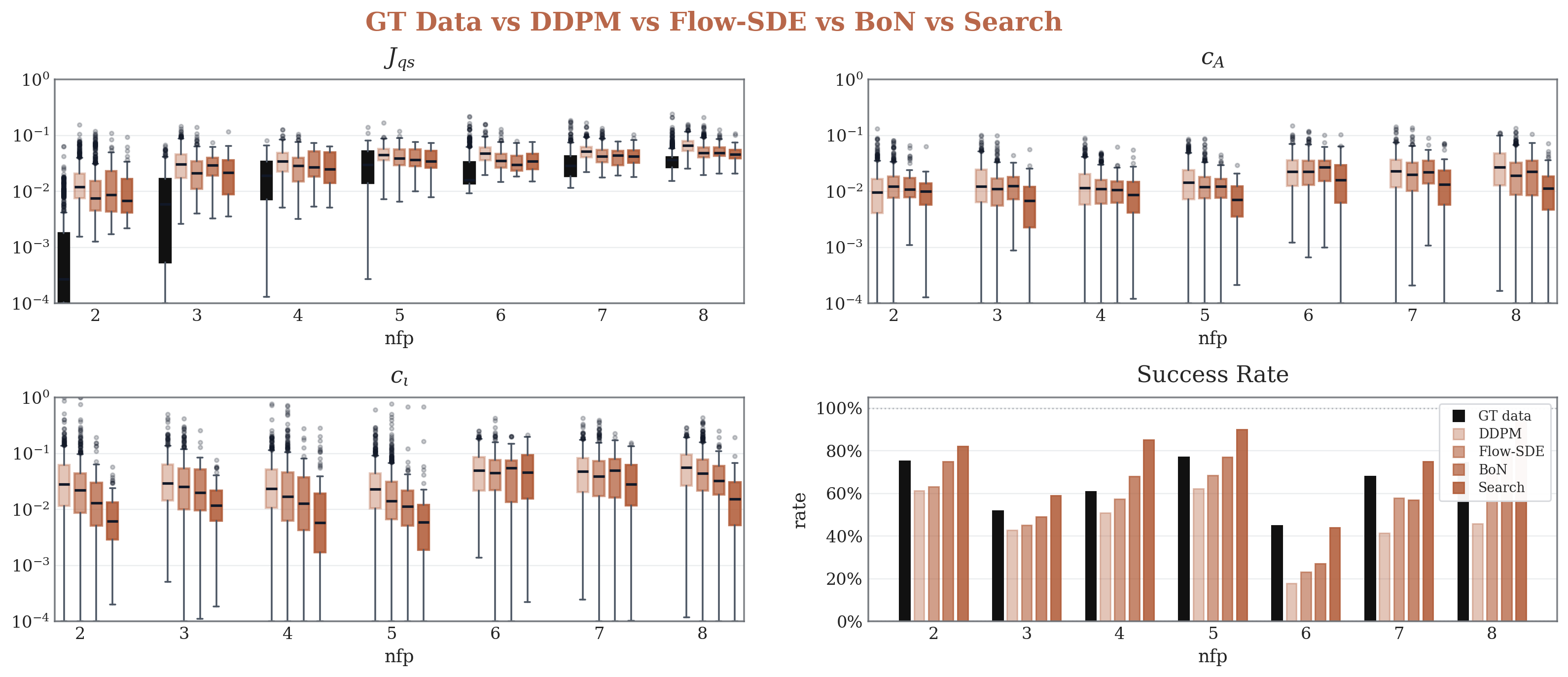
We compare the Flow-SDE search method with the Diffusion for Fusion DDPM baseline using the same physics-facing evaluation style.
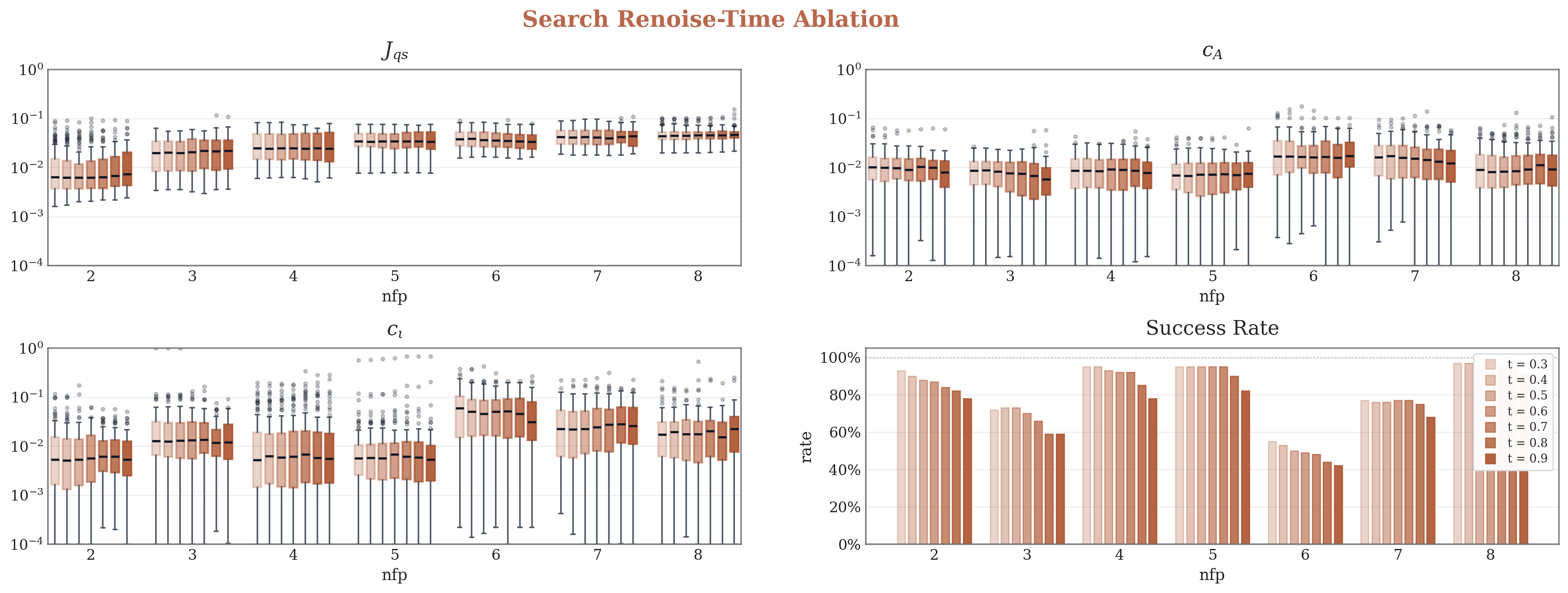
For the re-noising time ablation, we select $t=0.6$ and $t=0.8$ as balanced settings between local refinement and broader exploration.
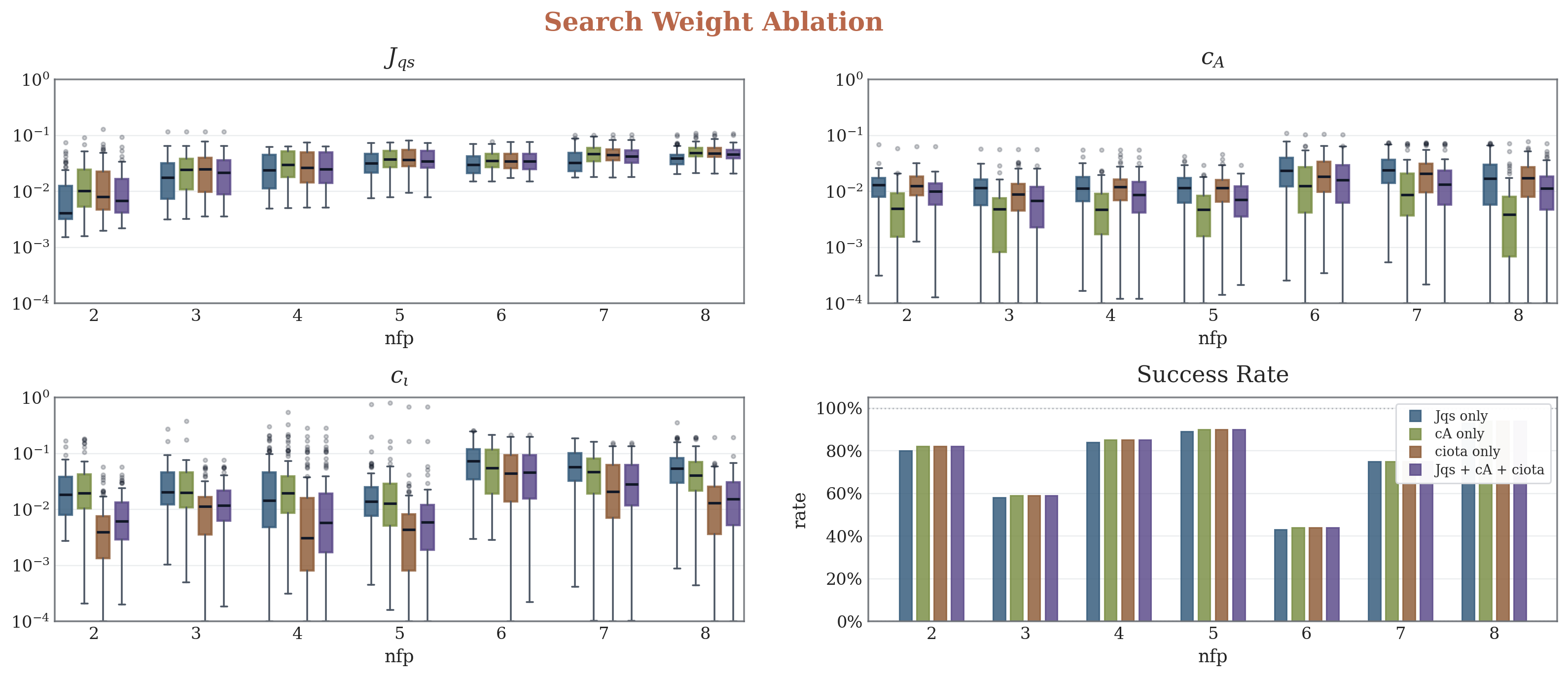
For the reward-weight ablation, emphasizing one reward term gives an obvious advantage on that term, while the trade-off appears across the other weighted objectives.
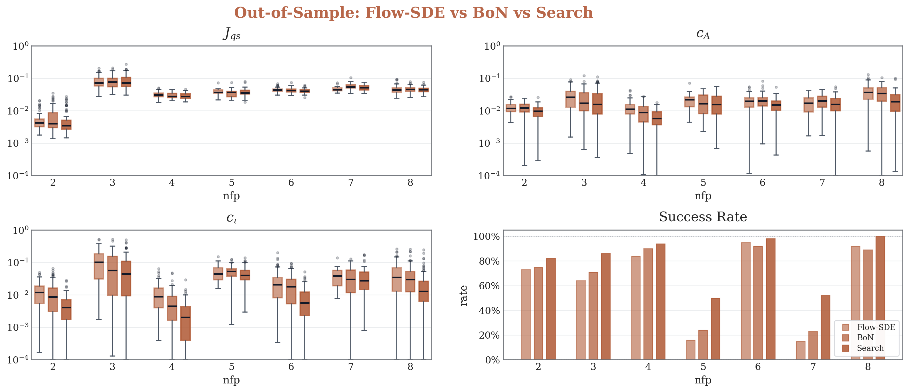
In the out-of-sample setting, the method improves $C_A$, $C_{\iota}$, and the success rate, while the improvement on $J_{\mathrm{qs}}$ is not yet obvious. We leave stronger out-of-distribution improvement in quasisymmetry quality to future exploration.
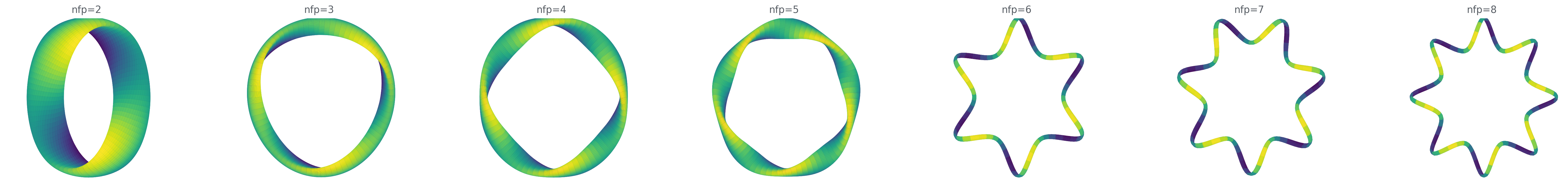
Here we also present the generated examples spanning 2-8 field periods.
Limitations and potential future directions
One limitation is evaluation cost. In the current experiments, we use 100 samples for comparison because VMEC evaluation is slow. For example, one search run can require $7 \times 100 \times (40+1)$ VMEC evaluations, which takes roughly three days to complete. This makes statistical noise unavoidable. To reduce the effect of a single noisy condition, we calculate the comparison across all $n_{\mathrm{fp}}$ settings when evaluating method effectiveness.
| Sample size | Success rate | $J_{\mathrm{QS}}$ |
|---|---|---|
| 10 | $76.7\% \pm 15.3\%$ | $0.046820 \pm 0.011268$ |
| 100 | $64.3\% \pm 2.5\%$ | $0.045189 \pm 0.001749$ |
| 1000 | $60.6\% \pm 1.4\%$ | $0.047211 \pm 0.000457$ |
| 5000 | $61.3\% \pm 0.7\%$ | $0.046627 \pm 0.000194$ |
Several extensions remain natural next steps. One direction is to examine whether the same formulation transfers beyond the current QA/QH setting based on QUASR-style data, especially toward QI configurations such as those represented in ConStellaration-style datasets